Simulation using Hspice

Hspice is an accurate and widely used simulator. It is worthwhile to take a look at some simple simulation using hspice. This tutorial will guide you through the windows version of the hspice. The linux version work on command line and should not me much different.

The input to hspice is a simple text file with .sp extention. This file contains a netlist of the circuit. Besides the netlist the same file has analysis options.

Let us take a look at the following hspice code.

* Stripline circuit
.Tran 50ps 7.5ns
.OPTION  post Probe
VIN 1 0 PWL 0 0v 250ps 0v 350ps 3.3v
Rsource 1 2 50
Tfirst 2 0 3 0 ZO=50 TD=0.17ns
*C2 3 0 2p
Tsecond 3 0 4 0 ZO=50 TD=500ps
Rtermination 4 0 50
.Probe v(1) v(2) v(3) v(4)
.End
 

Let us understand the elements of the code of hspice. The statement

* Stripline circuit

is a comment in hspice. Any line starting with * is taken as a comment. Use comments profusely to make your code more understandable.

The statement

.Tran 50ps 7.5ns

instructs hspice simulator to perform transient simulation analysis up to time period 7.5ns.

The statement

VIN 1 0 PWL 0 0v 250ps 0v 350ps 3.3v

Creates a piecewise linear voltage source. The voltage source is connected between nets named 1 and 0. The net 0 or GND is universally reserved for ground. At time t = 0, the level of voltage is 0v. At time t = 250 ps, the voltage level is 0v. At time t = 350 ps, the voltage level is 3.3v. This creates a voltage source with 0% to 100% rise time of 100 ps. The voltage rises between time 250 ps to 350 ps.

The statement

Rsource 1 2 50

connects a resistance of 50 ohm between net node 1 and net node 2. We therefore, have a voltage source with 50 ohm source resistance.

The statement

Tfirst 2 0 3 0 ZO=50 TD=0.17ns

Creates a transmission line connected between net node 2 and net node 3. The transmission line has a impedance of 50 ohms and delay of 0.17ns.

The statement

*C2 3 0 2p

is a comment. Had there been no * in the beginning it would have inserted a 2pf capacitor between net node 3 and ground.

The statement

Tsecond 3 0 4 0 ZO=50 TD=500ps

Again creates a transmission line of characteristic impedance 50 Ohms and length equivalent to a delay time of 500 ps.

We place a termination resistance of 50 Ohms, using the statement

Rtermination 4 0 50

Finally the statement

.Probe v(1) v(2) v(3) v(4)

is used to probe the voltage levels at nodes 1, 2, 3 and 4.

If we simulate the code and use Avanwaves to look at the waveforms, we should see something similar to the waveform below.



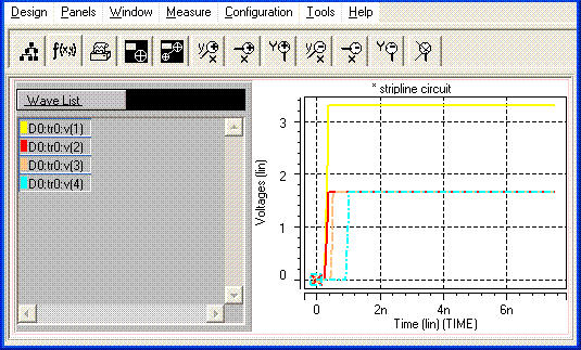
Figure Simple transmission line simulation in hspice.

The line with amplitude 3.3V shows the voltage source. It starts rising at t = 250 ps. It has a rise time of 100 ps. As soon as it passes the 50 Ohm series resistance and hits the first transmission line, its voltage level is halved according to the input acceptance voltage equation

v = viZo/(Zo+Zs).

As a result, a voltage level of 3.3V / 2 = 1.65 V starts propagating the first transmission line and the second transmission line. At the receiver, the waveform is completely absorbed in the 50 Ohm termination resistor and there is no reflection. The rightmost waveform shows the final waveform at node 4.


Previous - Chapter 9 - Question Answer                    Next - Hspcice - Reflected Wave Simulation