High Speed Characterization - Using Oscilloscope
OscilloscopeOscilloscope continues to form the major method for characterization of the high speed signals. All modern oscilloscopes come with ability to capture digitized waveform. When choosing an oscilloscope we must look for two important parameters. The first is the bandwidth. The bandwidth of the oscilloscope should be at least three times the highest frequency component of the signal we are willing to capture.
The bandwidth of an oscilloscope is related to rise time according to the equation
BW = 0.35 /Tr [12 1]
Where is the rise time. As an example let us assume that an oscilloscope is rated at 1G Hz. The rise time corresponding to this frequency is
Tr = 0.35 / ( 1GHz)
Or, Tr = 350 ps
It implies that if a signal with almost zero rise time is input to this oscilloscope, the oscilloscope will show a rise time of 350 ps.
If the rise time of the signal being observed is and oscilloscope has a rise time of Tr2, the rise time observed on the oscilloscope will be given by

Obviously, the oscilloscope slows down the edges. If we want to very accurately observe the signal we must have oscilloscope with bandwidth much higher than the frequency being observed.
Sometimes an oscilloscope comes with more than one probe options. The rise time of the scope and the probe are defined separately. If is the rise time of the signal being observed , is the rise time of Oscilloscope and is the rise time of the probe, then the rise time observed in the oscilloscope is given by

Where,
Tr1 = rise time of the signal
Tr2= rise time of Oscilloscope
Tr3=rise time of the probe
Tr= rise time observed in the oscilloscope
Another important parameter that we must look for in an oscilloscope is the number of samples per second that the scope can take. The higher the number of samples per second the scope can take, the better will be its resolution. There should be at least 3 samples during the rise time of the signal.
Example - A high end oscilloscope has designated bandwidth of 7 GHz. The rise time of a signal with this oscilloscope is observed to be 280 ps. Find the actual rise time of the signal.
Solution The rise time of the observed signal Tr is given by
Here Tr = 280 ps.
The rise time of the oscilloscope is given by
Tr2 = 0.35 / BW
= 0.35 / ( 7 GHz)
= 50 ps
Substituting the value of Tr and Tr2 in the equation
We get = 275 ps
The actual rise time of the signal was 275 ps.
Example - A high end oscilloscope has designated bandwidth of 7 GHz. The rise time of a signal with this oscilloscope is observed to be 80 ps. Find the actual rise time of the signal
Solution The rise time of the observed signal Tr is given by
Here Tr2 = 80 ps.
The rise time of the oscilloscope is given by
= 0.35 / BW
= 0.35 / ( 7 GHz)
= 50 ps
Substituting the value of Tr and Tr2 in the equation
We get = 62 ps
The actual rise time of the signal was 62 ps.
Note that the error becomes substantial if the rise time of the scope is close to the rise time of the signal under observation.
Sampling Rate Sampling rate of an oscilloscope refers to the number of samples it collects one second. Sampling rate determines the time interval between two samples. For example an 8 Giga samples per second oscilloscope captures samples every 125 ps.
If the sampling rate is insufficient, the oscilloscope will not be able to capture the artifacts in the signal. When capturing oscilloscope signals limitations due to the sampling rate must be kept in mind.
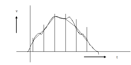
Figure An oscilloscope may miss glitches due to sampling rate limitation
The figure above shows an example of a signal having glitches in the rising and falling edge of the signal. The oscilloscope may not be able to capture these glitches due to the sampling rate limitation.
Time Domain Reflectometer
A Time Domain Reflectometer (TDR) can be used to measure the impedance and path loss of a lumped element or a transmission line. The TDR emits a short pulse, typically 25 ps. Let us assume that emitted pulse flows down a transmission line of infinite length or a transmission line terminated in its characteristics impedance. If there are no discontinuity along the path of the transmission line, there will be no reflection. The TDR screen will just show an incident signal. There will no signal from reflection.
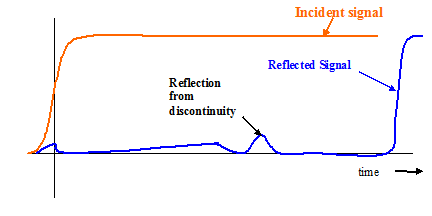
Now let us assume that a finite transmission line of say 10 inches in length is left open on the far end. If a short pulse is sent out to this transmission line, it will reach to the end of the transmission line and get reflected. The polarity of this reflected signal will be same as the incident signal. The two signals will add and travel back towards the TDR. The reflected signal can be observed in on the TDR screen.
TDR has been used in telephony to find the break positions of a cable. It has been used to detect and estimate the distance where the cable has possibly broken. This is done by calculating the distance using the formula c x t, where c is speed of the wave propagation in the medium and t is the time it takes to traverse the medium. A marker is placed at the launch time and another at the time when the reflected signal comes back from broken cable. The TDR screen shows waves as it traverses the cable and come back. By dividing the time between the launched signal and the reflected signal by 2 we get the time it took for the signal to reach from launches end to the broken end. Multiplying this time by the signal propagation velocity gives the distance.
In high speed digital designs, TDR is used to measure the characteristic impedance of traces. It can also be used to measure the values of lumped circuit element, for example, load capacitance of an IC.
Let us assume that a transmission line is terminated in a lumped element of impedance Zt.. As a result there is reflection from the end of the transmission line. The magnitude of the reflection is referred to as the reflection coefficient or ?. The reflection coefficient is calculated as follows: ρ= (Zt-Zo)/(Zt+Zo) Where Zo is defined as the characteristic impedance of the transmission medium and Zt is the impedance of the termination at the far end of the transmission line. ρ can be computed by taking the ratio of the incoming reflected signal with respect to the incident signal. We can then find the value of Zt. TDR can also be used to find the discontinuities along the transmission line as the signal propagates from one end of the transmission line to the other. At each discontinuity there will be reflection. These reflections can be observed on the TDR.
Previous Next